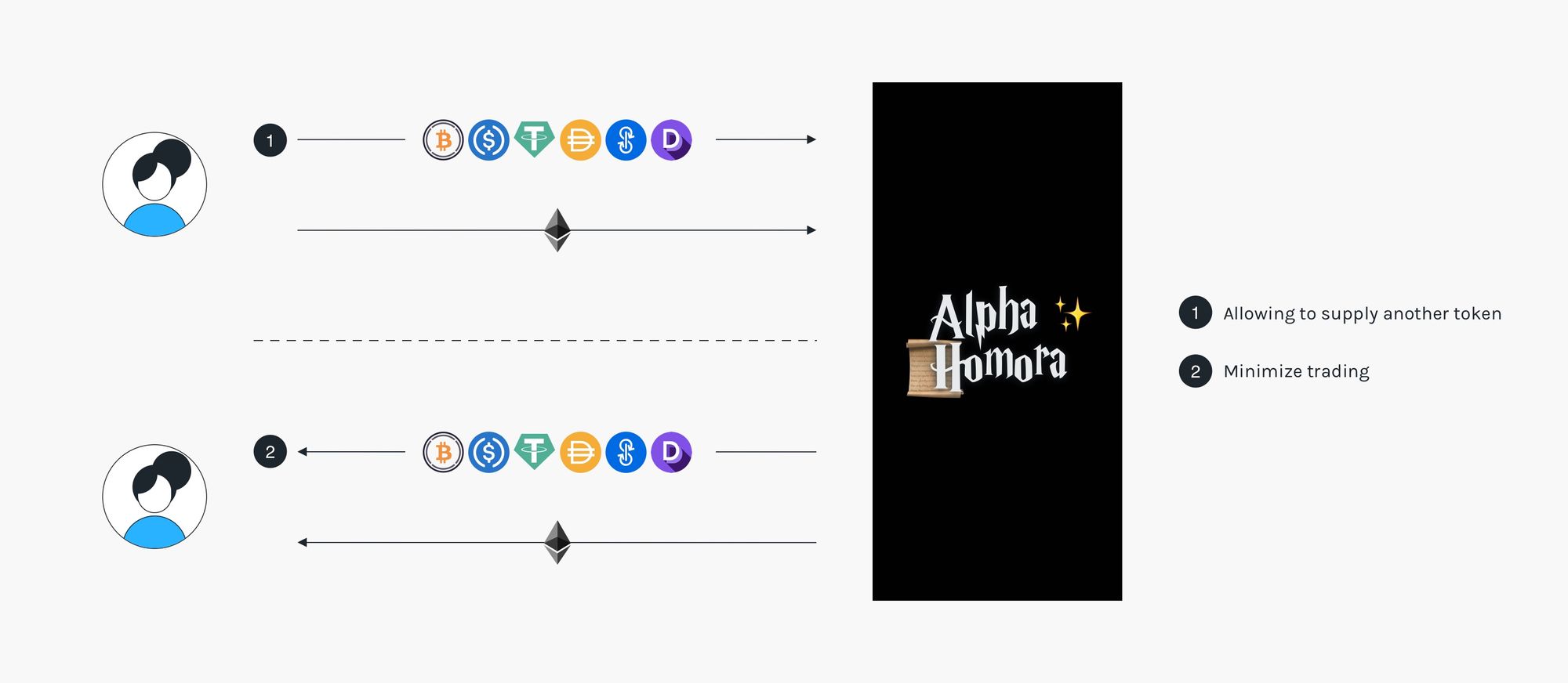
Alpha Homora Now Features Bring-Your-Own-Token (BYOT)

Alpha Homora now supports bring-your-own-tokens (BYOT) to yield farm \(\rightarrow\) minimize price slippage (as low as 0%)
\(\rightarrow\) maximize alpha!
How does it work?
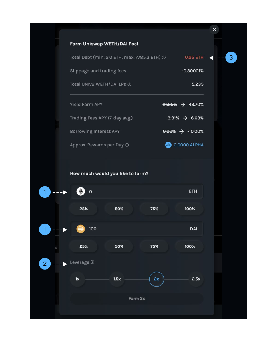
- Supply any amount of ETH and/or any amount of another token (DAI in the example above).*
- Specify leverage, borrowing the corresponding amount of ETH from the bank to farm.
- The protocol optimally swaps the tokens before supplying to the farming pool. In fact, the protocol doesn’t even need to swap in the example above, since 100 DAI is deposited and the corresponding 0.25 ETH is borrowed - supplying both DAI and ETH equally in value into Uniswap and reducing price slippage to 0%!
*Note: Previously, users can only supply ETH.
With this ‘bring-your-own-token’ (BYOT) feature in place and ‘Minimize Trading’ feature that we launched last week, Alpha Homora enables minimal slippage when opening a position (BYOT) while enabling minimal slippage when closing a position (Minimize Trading).
Alpha Homora continues to optimize for user experience and maximizes alpha through reducing slippage for users!
Example strategies and the math behind them
Here are some examples of the strategies this new feature enables (assuming Uniswap WETH/USDT pool has 70k ETH + 28M USDT, or ETH@400USDT):
Supply 1, Borrow 1 (Balanced Supply)
Currently only available for Uniswap's WETH/WBTC, WETH/USDT, WETH/USDC, WETH/DAI pools.
Get 0% price slippage.
Users supply 1 portion of farming tokens and also borrow 1 portion amount of ETH (2x leverage), getting 0% price slippage.
Ex:
- User's supply: 400k USDT
- Leverage: 2x (borrow 1k ETH)
- Swap required: 0 ETH (no swap needed \(\rightarrow\) 0% slippage)
- Total supply: 1k ETH + 400k USDT
Supply 2, Borrow 3
Currently only available for Uniswap's WETH/WBTC, WETH/USDT, WETH/USDC, WETH/DAI pools.
Get 5x lower price slippage.
Users can supply 2 portions of farming tokens and borrow 3 portions of ETH (2.5x leverage). Swapping required only on ~0.5 portion of ETH, lowering price slippage by ~5x (normally would need to swap ~2.5 portions of ETH to farming tokens).
Ex:
- User's supply: 400k USDT
- Leverage: 2.5x (borrow 1.5k ETH)
- Swap required: 0.25k ETH \(\rightarrow\) 100k USDT*
- Total supply: 1.25k ETH + 500k USDT
*Note: Previously, users are to supply 1k ETH and borrow another 1.5k ETH, then swapping ~1.25k ETH to USDT, which can incur 5x price slippage.
Supply 3.5+0.5, Borrow 3
Get 0% price slippage.
Users can supply 3.5 portions of farming tokens and 0.5 portions of ETH, and borrow 3 portions of ETH (1.75x leverage), getting 0% price slippage.
Ex:
- User's supply: 350k USDT + 0.125k ETH
- Leverage: 1.75x (borrow 0.75k ETH)
- Swap required: 0 ETH (no swap needed \(\rightarrow\) 0% slippage)
- Total supply: 0.875k ETH + 350 USDT
Supply 4, Borrow 3
Get 5x lower price slippage.
Users can supply 4 portions of farming tokens and borrow 3 portions of ETH (1.75x leverage). Swapping required only on ~0.5 portion of farming tokens, lowering price slippage by ~5x (normally would need to swap ~2.5 portions of ETH to farming tokens).
Ex:
- User's supply: 400k USDT
- Leverage: 1.75x (borrow 0.75k ETH)
- Swap required: 50k USDT \(\rightarrow\) 0.125k ETH*
- Total supply: 0.875k ETH + 350 USDT
*Note: Previously, users are to supply 1k ETH and borrow another 1.5k ETH, then swapping ~1.25k ETH to USDT, which can incur 5x price slippage.
Appendix
🚨 WARNING 🚨 : Heavy math involved.
For those interested in the math behind, here's a generalization to the previous blog to calculate the optimal swapping amount given that the users have both of the assets.
The two main questions are:
- Which direction should we swap the assets?
- What is the optimal swap amount?
Let's tackle the first problem.
Swap Direction (\(A \rightarrow B\) or \(B \rightarrow A \))
Suppose the two assets of interest are asset \(A\) and asset \(B\), and let's define some variables:
$$\begin{aligned}&res_A = \text{amount of asset \(A\) in the \(A\)-\(B\) pool reserve,} \\ &res_B = \text{amount of asset \(B\) in the \(A\)-\(B\) pool reserve,} \\ &amt_A = \text{amount of asset \(A\) the user wants to supply optimally, } \\ &amt_B = \text{amount of asset \(B\) the user wants to supply optimally, and}\end{aligned}$$
Clearly, if the user has "too many" of asset A, then the user should swap from \(A \rightarrow B\). Otherwise, the user should swap from \(B \rightarrow A\). The breakpoint is when the user's asset ratio matches the reserve's asset ratio, i.e., \(\frac{amt_A}{res_A} = \frac{amt_B}{res_B}\). In this case, the user can simply deposit both of the assets optimally. Hence,
$$\text{swap direction} = \begin{cases} &A \rightarrow B, \text{ \hspace{5ex} if \(\frac{amt_A}{res_A} > \frac{amt_B}{res_B}\), } \\ &\text{no swap}, \text{\hspace{5.3ex} if \(\frac{amt_A}{res_A} = \frac{amt_B}{res_B}\), and} \\ &B \rightarrow A, \text{ \hspace{5.5ex} if \(\frac{amt_A}{res_A} < \frac{amt_B}{res_B}\).} \end{cases} $$
For simplicity, the rest of the article assumes \(\frac{amt_A}{res_A} \ge \frac{amt_B}{res_B}\) (swapping \(A\rightarrow B\), possibly zero amount swap). The other case can be done similarly by symmetry.
Knowing the swap direction, we can now move on to find the optimal swap amount.
Optimal Swap Amount
This section follows closely to the previous blog but with a more complex calculation.
Assume the defined variables from the previous section, condition \(\frac{amt_A}{res_A} \ge \frac{amt_B}{res_B},\) and further define
$$\begin{aligned}f = \text{swap fee (0.3\% for Uniswap).} \end{aligned}$$
The goal of this section is to find the optimal \(swapAmt_A\) to get a corresponding amount of asset B, so that the proportion of assets the user holds is equal to the proportion of assets in reserves after swap. We again proceed in 2 steps:
- calculating the amount of asset \(B\) received from swap, and
- the user's asset ratio should now be the same as reserve's after the swap.
Calculating the amount of asset \(B\) received
The initial constant product is given by
$$k = res_A \cdot res_B.$$
According to Uniswap's implementation, swap fee is deducted from input asset amount, so the new \(res'_B\) should satisfy:
$$ k = (res_A + (1-f) \cdot swapAmt_A)\cdot res'_B. $$
This means the user will receive amount of asset \(B\) equal to
$$ \begin{aligned} rcvAmt_B &= res_B - res'_B \\ &= res_B - \frac{k}{res_A + (1-f)\cdot swapAmt_A} \\ &= res_B - \frac{res_A \cdot res_B}{res_A + (1-f)\cdot swapAmt_A} \\ &= \frac{(1-f)\cdot swapAmt_A \cdot resB}{res_A + (1-f)\cdot swapAmt_A}.\end{aligned} $$
User's asset ratio = reserve's asset ratio
The optimal \(swapAmt_A\) should satisfy the equality constraint on user's asset ratio and reserve's asset ratio:
$$\begin{aligned} \frac{amt_A - swapAmt_A}{amt_B + rcvAmt_B} = \frac{res_A + swapAmt_A}{res'_B}. \end{aligned}$$
Substituting known variables \(rcvAmt_B\) and \(res'_B\), and rearranging the equation yields a quadratic equation in variable \(swapAmount_A\) as follows:
$$\begin{aligned}&\Big((1-f)\cdot (amt_B + res_B)\Big)\cdot (swapAmt_A)^2 \\ &+ \Big((2-f)\cdot (amt_B + res_B) \cdot res_A\Big) \cdot swapAmt_A \\ &- \Big(amt_A \cdot res_A \cdot res_B - amt_B \cdot res_A^2\Big) = 0.\end{aligned}$$
Solving for \(swapAmt_A\)
Solving the above equation for a non-negative root yields:
$$\begin{aligned} swapAmt_A = \frac{\sqrt{\Big((2-f)\cdot res_A\Big)^2 + \frac{4(1-f) \cdot res_A\cdot (amt_A \cdot res_B - amt_B \cdot res_A)}{ amt_B + res_B }} - (2-f) \cdot res_A}{2(1-f) },\end{aligned}$$
where we are guaranteed \(amt_A \cdot res_B - amt_B \cdot res_A \ge 0\) from our assumption \(\frac{amt_A}{res_A} \ge \frac{amt_B}{res_B}\).
Note: When \(amt_B = 0\), the equation is exactly the same as the one-sided liquidity equation.
Implementation Practicality
There are 2 main concerns for this formula in actual implementation:
- Floating-point calculation
uint256size limit (max value of ~\(10^{77}\))
Floating-point Calculation
When \(f\) = 0.003, we can avoid floating point numbers by multiplying both the numerator and the denominator by 1000.
uint256 size limit
Uniswap protocol assumes a maximum number of token in the pool to be at most \(2^{212} \approx \)We assume a standard token has a maximum of one trillion \(10^{12}\) token supply with \(10^{18}\) decimals; otherwise, it's most likely a scam. So, we assume the maximum token amount in its smallest unit is at most \(10^{12} \cdot 10^{18} = 10^{30}\).
Thus, a single uint256 (max value of ~\(10^{77}\)) can only fit a quadratic expression of amounts of tokens. However, our formula contains the term (inside the big square root)
$$\frac{4(1-f) \cdot res_A\cdot (amt_A \cdot res_B - amt_B \cdot res_A)}{ amt_B + res_B }, $$
which is cubic in the numerator.
Our solution
We use the following formula:
$$\begin{aligned} swapAmt_A = \left\lfloor\frac{\left\lfloor\sqrt{1997^2\cdot res_A^2 + 4\cdot 997\cdot 1000 \cdot res_A\cdot \left\lfloor\frac{amt_A \cdot res_B - amt_B \cdot res_A}{ amt_B + res_B }\right\rfloor}\right\rfloor - 1997 \cdot res_A}{1994 }\right\rfloor.\end{aligned}$$
The question now is how large can the difference between the actual value and the rounding value be.
\(swapAmt_A\) Rounding Error Estimation
Let's first provide a bound on \(swapAmt_A\) rounding.
From the formula, each of the two outer floor functions clearly contribute at most value of \(1\) to the difference, so the largest possible error from the outer floors can be at most 2 (in the smallest unit of token).
What about the innermost floor function? The error is bounded by the difference between:
$$\begin{aligned} &\frac{\sqrt{1997^2\cdot res_A^2 + 4\cdot 997\cdot 1000 \cdot res_A\cdot \frac{amt_A \cdot res_B - amt_B \cdot res_A}{ amt_B + res_B }} - 1997 \cdot res_A}{1994 } \\ &- \frac{\sqrt{1997^2\cdot res_A^2 + 4\cdot 997\cdot 1000 \cdot res_A\cdot \left\lfloor\frac{amt_A \cdot res_B - amt_B \cdot res_A}{ amt_B + res_B }\right\rfloor} - 1997 \cdot res_A}{1994 },\end{aligned}$$
or equivalently,
$$\begin{aligned} \frac{1}{1994}\Bigg(&\sqrt{1997^2\cdot res_A^2 + 4\cdot 997\cdot 1000 \cdot res_A\cdot \frac{amt_A \cdot res_B - amt_B \cdot res_A}{ amt_B + res_B }} \\ &- \sqrt{1997^2\cdot res_A^2 + 4\cdot 997\cdot 1000 \cdot res_A\cdot \left\lfloor\frac{amt_A \cdot res_B - amt_B \cdot res_A}{ amt_B + res_B }\right\rfloor} \Bigg).\end{aligned}$$
Let \(X\) and \(Y\) be the expression inside the first and the second square-root in the above expression, respectively. Using the conjugation and the fact that \(X \ge Y\), we get
$$\frac{1}{1994}(\sqrt{X} - \sqrt{Y}) = \frac{1}{1994}\left(\frac{X-Y}{\sqrt{X} + \sqrt{Y}}\right) \le \frac{1}{1994}\left(\frac{X-Y}{ 2\sqrt{Y}}\right). $$
Now, by floor function property,
$$\begin{aligned}X-Y &= 4\cdot 997\cdot 1000 \cdot res_A\cdot\left\{\frac{amt_A \cdot res_B - amt_B \cdot res_A}{ amt_B + res_B }\right\} \\ &\le 4\cdot 1997 \cdot 1000 \cdot res_A, \end{aligned}$$
where \(\{x\}\) denotes the fractional part of \(x\). Together with the lower-bound \(Y \ge 1997^2 \cdot res_A^2\), it follows that
$$\begin{aligned} \frac{1}{1994}(\sqrt{X} - \sqrt{Y}) &\le \frac{1}{1994}\left(\frac{X-Y}{ 2\sqrt{Y}}\right) \\ &\le \frac{1}{1994}\left(\frac{4\cdot 1997 \cdot 1000 \cdot res_A}{2\sqrt{1997^2 \cdot res_A^2}}\right) \\ &< 2 . \end{aligned}$$
Thus, we can conclude that
$$\text{RoundingError}({swapAmt_A}) < 4.$$
A Bound on the Value of Remaining Amount after Supply
With rounding, the \(swapAmt_A\) can be off by at most 4 minitokens, but how large can the remaining user's balance be after supply? We omit a formal proof here, but it can easily be shown that the amount is bounded by the order of the exchange rate, i.e., 1 minitoken of one asset is equivalent to how many minitokens of another asset.
The remaining value is then bounded by 4 minitokens of the greater-value asset, which should still be insignificant for standard assets.
Note: The remaining amount of minitokens of lesser-value asset can be fairly large due to extreme exchange rate, but the value should still be in the order of 4 minitokens of the greater-value asset.
How does this complex formula look in real implementation?
Again, using the Babylonian method to compute the square root, it's easy to compute the optimal swap amount:
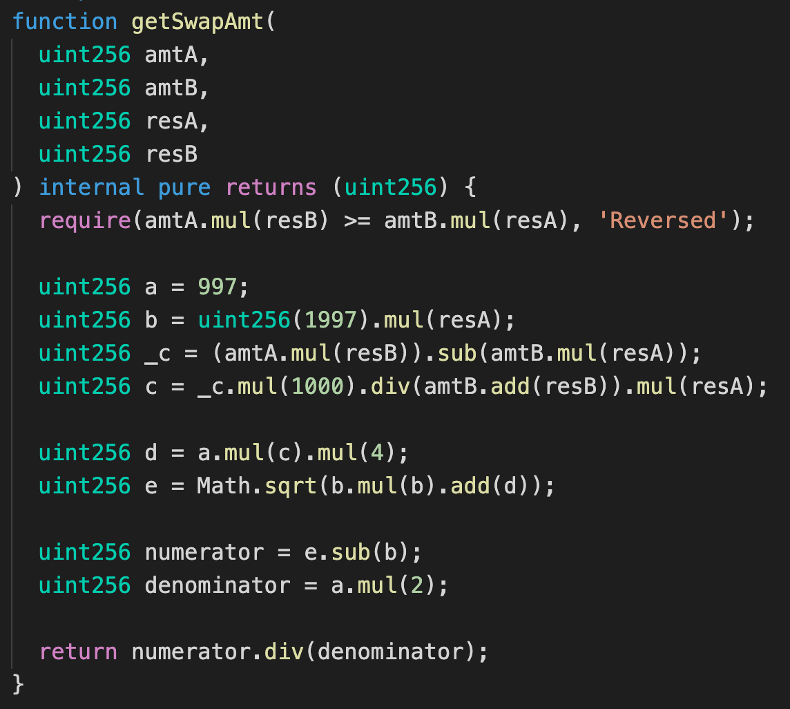
Note: The square root implementation is from UniswapV2 library.
In Conclusion...
We have presented an algorithm to optimally supply two-sided assets to the Uniswap pool. The formula even also be used in similar protocols with different swap fee \(f\). The article also shows that the algorithm is efficient, not utilizing at most only a very insignificant remaining value of assets.
Follow AlphaFinanceLab on Twitter or join our community on Discord to hear our latest news and updates!