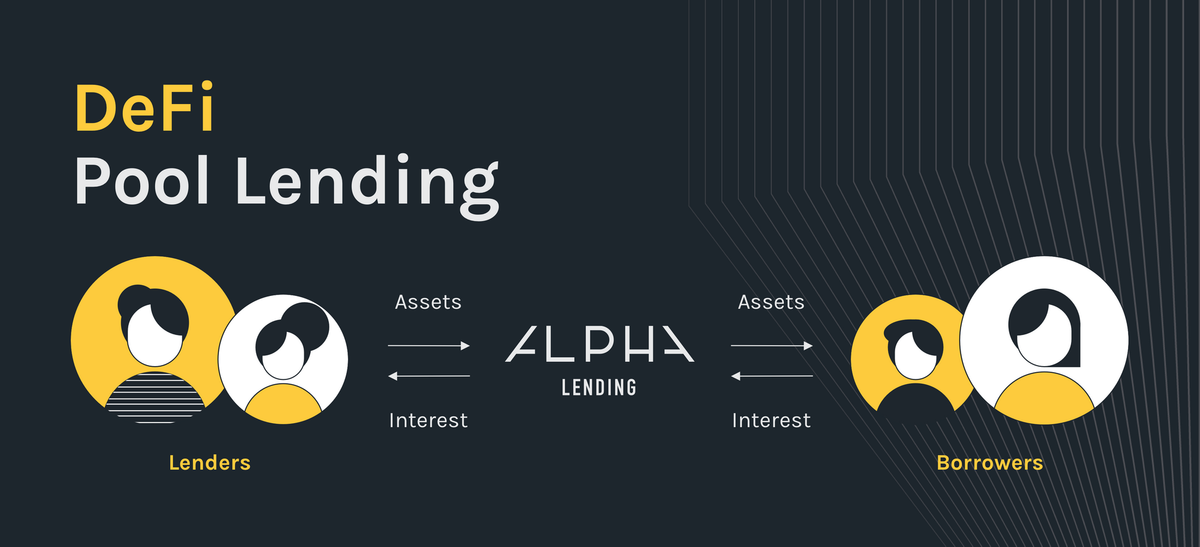
DeFi Pool Lending

In the decentralized finance (DeFi) space, many lending protocols such as Aave, Compound, dYdX, and C.R.E.A.M. have recently gained so much popularity that the total value locked (TVL) across these protocols is worth multi-billion of dollars.

The success of DeFi lending lies in anonymity. Any user can lend/borrow assets while earning/paying the corresponding interest rates without any centralized third-party or any know-your-customer (KYC) verification.

Two currently popular lending protocols are flash loans and pool lendings (at the time of writing).

• Flash loan - Ethereum virtual machine (EVM) allows the concept of "instantaneous borrowings," where borrowers can simply borrow assets and return the borrowed amount within a single transaction; the whole transaction gets reverted if the returned amount is less (borrowers only pay gas fees).
• Pool lending - Unlike traditional lending where lenders and borrowers need to be matched and then form contracts, both parties instead interact with a common asset pool. Lenders' and borrowers' interest rates are automatically determined by each asset's borrowing to lending ratio.

The rest of the article will focus only on the insights behind the pool lending protocols, including possible areas of improvements.

Key Terms & Components

Let's first go through commonly used terms, symbols, and components.

Lending protocol's entities include

• Lender - A user who lends his/her assets.  
• Borrower - A user who borrows assets. Note: A user can be simultaneously be both a lender and a borrower (of different assets).
• Liquidity Pool (LP) - Common asset pool (e.g., DAI pool, USDT pool, ETH pool) where lenders deposit to and borrowers withdraw from. Note: Different assets will have different LPs.

Asset-level values include

• \(LendInterestRate_{a}\) - Interest rate* a lender gains from lending asset \(a\).
• \(BorrowInterestRate_{a}\) - Interest rate* a borrower must pay from borrowing asset \(a\).
• \(Price_{a, t}\) - Price of the asset \(a\) at time \(t\).
• \(BorrowAmount_{a, u, t}\) - Borrowed amount of asset \(a\) by user \(u\) at time \(t\).
• \(LendAmount_{a, u, t}\) - Lent amount of asset \(a\) by user \(u\) at time \(t\).
• \(ReserveFactor_{a}\) - The reserve factor of asset \(a\) for lenders' insurance.
• \(U_{a,t}\) - Utilization rate of asset \(a\) at time \(t\).
• \(U_{opt, a}\) - Optimal utilization rate of asset \(a\).
• \(CollateralFactor_{a}\) - How much of the value of asset \(a\) can actually be used as collateral.
• \(AssetBorrowAmount_{a,t}\) - Total borrowed amount of asset \(a\) across all users at time \(t\). $$AssetBorrowAmount_{a,t} = \sum_{User\; u} BorrowAmount_{a, u, t}.$$
• \(AssetLendAmount_{a,t}\) - Total lent amount of asset \(a\) across all users at time \(t\). $$AssetLendAmount_{a,t} = \sum_{User\; u} LendAmount_{a, u, t}.$$
• \(AssetLiquidityAmount_{a,t}\) - Total available liquidity of asset \(a\)  at time \(t\), not including asset total reserves.
• \(LiquidationBonus_{a}\) - Liquidation bonus given to liquidators to get better-than-market prices as incentives to clear accounts at risk of going underwater.

*Note: Most implementations calculate interest rates as compounded per block. For example, if the interest rate is \(I\) per year, then on EVM  with \(N\sim 2\cdot 10^6\) blocks per year, the actual annual interest rate collected will be
$$\left(1+\frac{I}{N}\right)^N - 1\approx e^I - 1.$$ This exponential value grows at a higher rate than the interest rate \(I\). So, borrowers will actually pay higher interest rate than specified in \(BorrowInterestRate_{a}\).

LP-level values include

• \(TotalReserve_{a,t}\) - Total reserve of asset \(a\) at time \(t\).
• \(UserBorrowAmount_{u,t}\) - Total borrowed amount of user \(u\) across all assets at time \(t\). $$UserBorrowAmount_{u,t} = \sum_{Asset\; a} BorrowAmount_{a, u, t}.$$
• \(UserLendAmount_{u,t}\) - Total lent amount of user \(u\) across all assets at time \(t\). $$UserLendAmount_{u,t} = \sum_{Asset\; a} LendAmount_{a, u, t}.$$
• \(TotalBorrowAmount_{t}\) - Total borrowed amount across all assets and all users at time \(t\). $$TotalBorrowAmount_{t} = \sum_{User\; u} UserBorrowAmount_{u, t}.$$
• \(TotalLendAmount_{t}\) - Total lent amount across all assets and all users at time \(t\). $$TotalLendAmount_{t} = \sum_{User\; u} UserLendAmount_{ u, t}.$$
• \(TotalLiquidityAmount_{t}\) - Total available liquidity across all assets at time \(t\), not including asset total reserves.
• \(UserCollateralValue_{u,t}\) - Total value of collaterals of user \(u\) at time \(t\).
• \(AccountHealth_{u,t}\) - Ratio of total  for user \(u\) at time \(t\). If value falls below 1, the user's collaterals can be liquidated. $$H_{u,t} = \frac{UserCollateralValue_{u,t}}{UserBorrowAmount_{u,t}}.$$

Now that we have defined some core terminology, we would like to provide insights to the protocol's relationships and constraints on these variables to make the model efficient.

Protocol Key Requirements

Here are some requirements for the lending protocol to succeed:

1. Borrowers should pay interests, which should cover interests gained by lenders. That is,
   $$\begin{aligned}&LendInterestRate_{a} \cdot AssetLiquidityAmount_{a,t} \\ &\le BorrowInterestRate_{a} \cdot AssetBorrowAmount_{a,t}, \end{aligned}$$ or equivalently,
   $$\begin{aligned}LendInterestRate_{a} &\le \left(\frac{AssetBorrowAmount_{a,t}}{ AssetLiquidityAmount_{a,t}} \right)\cdot BorrowInterestRate_{a} \\ &= U_{a,t} \cdot BorrowInterestRate_{a}.\end{aligned}$$
   The ratio \(U_{a,t} = \frac{AssetBorrowAmount_{a,t}}{AssetLiquidityAmount_{a,t}}\) defines the proportion of the liquidity borrowed, thus the utilization rate of asset \(a\).
   
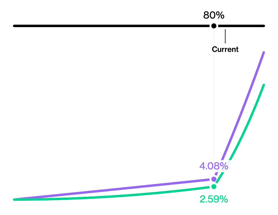
   The higher the utilization rate, the higher the lenders gain. However, if the rate is too high, lenders are more at risk when prices fluctuate. Thus, an asset's optimal utilization rate \(U_{opt,a}\) should balance between risks and rewards.
   
   To incentivize lenders and borrowers to maintain utlilization rate at optimal, double-slope interest rate curve is commonly adopted. Initially slow increase in interest rate incentivizes borrowing at low rate, while sharp rise beyond optimal point discourages borrowers keep utilization rate lower than optimal.
2. At any time \(t\), any user \(u\) should have the total lent value of at least the total borrowed value. That is,
   $$\begin{aligned}&\sum_{Asset\; a} LendAmount_{a,u,t} \cdot Price_{a,t} \\ &\ge \sum_{Asset\; a} BorrowAmount_{a,u,t} \cdot Price_{a,t}.\end{aligned}$$

These two requirements are bare-minimum to guarantee that lenders have the sufficient incentives to provide liquidity to the pool and that borrowers are better off not defaulting.

But how to enforce requirements to hodl under volatile prices?

In practice, volatile asset prices can easily cause the total borrowed value to exceed the total collateral values. Thus, most protocols assign collateral value for each asset as a safety buffer. The more volatile the prices are, the lower the collateral values will be.

Requirement (2.) becomes:

2.1 At any time \(t\), any user \(u\) should have the total collateral value of at least the total borrowed value. $$\begin{aligned}&\sum_{Asset\; a} CollateralFactor_{a} \cdot LendAmount_{a,u,t} \cdot Price_{a,t} \\ &\ge \sum_{Asset\; a} BorrowAmount_{a,u,t} \cdot Price_{a,t}.\end{aligned}$$ Whenever (2.1) fails to hold, any user can liquidate the user's collaterals to clear these debts at risk at a discounted price.

Still, what if liquidators did not liquidate in time?

In this scenario, borrowers are likely to default the loan since their collateral values are of less value. The LP has thus acquired pool debt. One mitigation is to set up reserve for each asset to cover these small debts. A portion of borrowers interests go into reserves, based on reserve factor \(ReserveFactor_{a} < 1\).

Possible Areas of Improvements

Although many popular contracts follow the core concepts of pool lending described above, here are some areas that can potentially provide the model more efficiency:

• Interest Rate Model - what other models (apart from double-slope curve) can be used that would still incentivize high utilization rate while balancing underwater risk?
• Constants - how can we make constants, including optimal utilization rate \(U_{opt}\), collateral ratio \(CollateralFactor_{a}\), reserve factor \(ReserveFactor_{a}\), make lending and borrowing more efficient. These values may differ from contracts to contracts, but what values will be the most efficient?
• Asset Prices - how to obtain accurate and up-to-date market price for each asset? E.g., centralized exchange, and decentralized price oracle.
• Are there any alternative mitigations to using safety buffers like collateral factors.

We will dig into and discuss some of these areas in future articles. Stay tuned!

Follow AlphaFinanceLab on Twitter or join our Telegram channel!